Fitting post processing

In this notebook it is demonstrated how to work with the result file generated by the fitter

Diagnostic plotting is shown, as well as the construction of deviation plots, and so on

General notes:

• To keep the approach flexible, each of the plotting routines assumes that an axis is already prepared for plotting. This allows you to make complex grids of axes and plot different things (different model results) in each axis.

• For other plots that do not generalize as easily, example plots are shown demonstrating the workflow generally

import os
import matplotlib.pyplot as plt
from temo.analyze.plotting import ModelAssessmentPlotter, PairMinFilter, ResultsParser

from temo.fit.cost_contributions import calc_errrho
from temo.fit.data_loaders import _density_processing, only_the_fluids
import CoolProp.CoolProp as CP

# Files in this folder, make sure we have the desired fitting result file
os.listdir()

['index.rst',
 'runc709530e-e431-11ed-b7b3-8e94f88bf11a.tar.xz',
 'FittingPostProcessingPlotting.ipynb']

run_file = 'runc709530e-e431-11ed-b7b3-8e94f88bf11a.tar.xz'
# Let's see what results we obtained
rp = ResultsParser(run_file)
# Show the pandas.DataFrame; bigger jobs can have MANY entries, several different pairs, etc.
rp.dfresults

./c709cf8c-e431-11ed-b7b3-8e94f88bf11a.json

	model	cost	pair	Ndep	uid	bounds	mutant_kwargs	x	elapsed / s
0	{'0': {'1': {'BIP': {'Fij': 1.0, 'betaT': 1.00...	1.003476	[R32, R1234YF]	3	c709cf8c-e431-11ed-b7b3-8e94f88bf11a	[[0.75, 1.25], [0.75, 1.25], [0.75, 1.25], [0....	{'Npoly': 3, 'Ngaussian': 0, 'd': [1, 1, 1], '...	[1.0063665465492047, 0.9590637406962529, 0.998...	342.416965

# And now we start plotting, first by filtering by pair to find the pair run
# with the lowest value of the cost function, which we can assume is the
# best optimization run
mapp = ModelAssessmentPlotter(
    result_path=run_file,
    result_filter=PairMinFilter(['R32',"R1234YF"])
)

./c709cf8c-e431-11ed-b7b3-8e94f88bf11a.json

# First thing to make sure the run is converged,
# at least approximately, so we plot the cost function
# history
fig, ax = plt.subplots()
comps = [0.3, 0.7]
mapp.plot_cost_history(ax=ax, stepfiles=mapp.stepfiles)

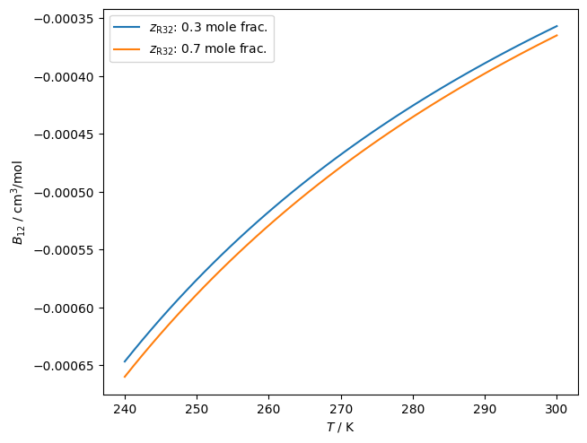
# Next we plot the B12 for two compositions, to make sure
# that they are close to the same
fig, ax = plt.subplots()
comps = [0.3, 0.7]
mapp.plot_B12(ax=ax, z1_comps=comps, Trange=(240, 300),
              labels=[rf'$z_{{\rm R32}}$: {z} mole frac.' for z in comps])
# <USER>
# And you could add experimental data points here...
# </USER>
plt.tight_layout(pad=0.2)

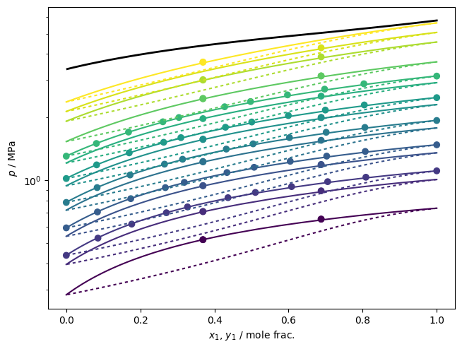
# A pretty colored p-x diagram
fig, ax = plt.subplots()
comps = [0.3, 0.7]
# First plot the points from the fitting data file
# Note: you can pass keyword arguments to the
# read_csv function here if needed
df = mapp.results.get_fitdata_df(key='VLE', sep=',')
sc = ax.scatter(x=df['x_1 / mole frac.'], y=df['p / kPa']/1e3, c=df['T / K'])
# Then plot the corresponding isotherms with matching color scheme
ipure = 0
mapp.plot_binary_VLE_isotherms(
    ax=ax, Tvec=set(df['T / K']), cmap=sc,
    ipure=ipure, basemodel=mapp.basemodels[ipure]
)
# And the critical locus too for good measure
mapp.plot_binary_critical_locus(
    ax=ax, ipure=ipure, kind='XP',
    options={'rel_err': 1e-10},
    plot_kwargs={'color': 'k', 'lw': 2}
)
plt.tight_layout(pad=0.2)
plt.show()

# Extract the data file from the archive
df = mapp.results.get_fitdata_df(key='PVT')
df['phases'] = 'FL'
df['property'] = 'VDM'
df.dropna(inplace=True, subset={'T / K'})

# Subset to the pair of interest
df = only_the_fluids(df, identifier='FLD', identifiers=mapp.pair)

# Add molar density
molar_masses = [CP.PropsSI('molemass', F) for F in mapp.pair]
df = _density_processing(df, molar_masses=molar_masses)

# Calculate the deviations with the best model
df['Deltarho / %'] = calc_errrho(df=df, model=mapp.model, iterate=False)
# df.to_csv('data.csv', index=False)

fig, (axT, axD) = plt.subplots(1, 2)
axT.plot(df['T / K'], df['Deltarho / %'], 'o')
axD.plot(df['rho / mol/m^3'], df['Deltarho / %'], 'o')
axT.set_xlabel('T / K')
axT.set_ylabel(r'$\Delta\rho/\rho\times 100$')
axD.set_xlabel(r'$\rho$ / mol/m$^3$')
plt.show()